Introduction to Machine Learning

Machine Learning is tightly coupled with Data Science, and is for the most part a data-driven field. It’s chiefly concerned with taking some initial data set as a starting point and using it to predict the properties of unknown data. As such, Machine Learning problems tend to come in two flavors: Classification and Regression

Machine Learning Problems

Classification

The main statement: Data from the same population should share similar characteristics that differentiate them from other populations. Thus given some data, we should be able to adequately categorize some new data.

For example:

• Teenagers tend to have fewer financial assets and know fewer people than thirty-somethings.
• Sea water near the equator has higher temperatures and lower mineral content than water near the poles.
• Public schools tend to have larger class sizes, lower test scores, and less funding than private schools.

Regression

The main statement: While it may not be simple, the world acts in a predictable, regular manner. So, given data on the way that a certain thing has been behaving thus far, I can predict how it will behave in the future.

For example:

• Stock market (or Bitcoin) prices with time
• The average width of a tree’s leaf given the height of the tree
• Activity on Twitter given the hour of the day

Whether attacking an issue of classification or regression, a Machine Learning problem will require data to make decisions. Python’s scientific and numerical tools allow us to read, write, visualize, and otherwise work with this data in an efficient and organized manner. Typically those tools are wrapped together and included in the Anaconda distribution of Python. DO NOT DOWNLOAD THIS DISTRIBUTION. IT WILL WRECK YOUR WORK WITH ENVIRONMENTS.

Instead follow these steps:

bash-3.2$ mkdir machine_learning
bash-3.2$ cd machine_learning
bash-3.2$ python3 -m venv ENV
bash-3.2$ source ENV/bin/activate

Download the tools in the requirements file here to your new machine_learning directory. Then, pip install the requirements file:

(ENV) bash-3.2$ pip install -r data_science_requirements.txt --upgrade

Jupyter Notebook

Thus far we’ve written all of our Python code either in scripts or on the command line using the Python interpreter. Jupyter notebooks combine the convenience and code-persistence of the iPython interpreter with the editability and thought-persistence of a script. The file extensions for Jupyter notebooks are .ipynb since they inherit from what used to be iPython notebooks. Let’s create one!

(ENV) bash-3.2$ jupyter notebook
[I 17:24:55.837 NotebookApp] Serving notebooks from local directory: /Users/Nick/Documents/codefellows/courses/code401_python/machine_learning
[I 17:24:55.838 NotebookApp] 0 active kernels
[I 17:24:55.838 NotebookApp] The Jupyter Notebook is running at: http://localhost:8888/
[I 17:24:55.838 NotebookApp] Use Control-C to stop this server and shut down all kernels (twice to skip confirmation).

Unless told otherwise (or there’s another instance of Jupyter Notebook already running), Jupyter Notebook will always serve on port 8888. Jupyter Notebook will pop open a tab in your browser at the address http://localhost:8888/tree where you will see your current working directory. In it will be all the files you currently have access to.

We can create a new notebook using the menu on the right side of the screen. Click the “New” button to get a dropdown menu and Python 3 to open a new Python 3 Jupyter Notebook. If your environment also included Python 2, you’d have the option to open a notebook in Python 2.

When you open a new notebook you’re started off with an empty cell. Within this cell you will write code as you would either in a script file or in the command line. The code that you write will automatically have syntax highlighting for your convenience. You execute the code within a cell by holding Shift and pressing Enter.

In [1]: print("Hello World")
Hello World

If the line of code that you write prints to stdout, that output will appear below the cell. If instead you declare a variable, import anything, or declare a function or a class, nothing will appear. You can of course write multiple lines of code, because otherwise it’d just be silly.

You can write code in your notebook as you would in any script file. If you try to write code blocks, it will auto-indent for you. Some of the same commands for applying comments or indentations in Sublime (or Atom) are present here.

If you need to check the documentation of an object or method, type the following

In [2]: ? object_or_method

Jupyter Notebook will pop up a mini-window from the bottom of your screen containing the top-level documentation for that object or method. You can also get more detailed documentation by typing

In [3]: help(object_or_method)

Jupyter will print the detailed documentation for you below that cell in a scrollable field.

One important difference between Jupyter Notebook and iPython is that the order in which code is executed can change and is extremely important. Consider the line numbers on the left side. The higher the number, the more recently that cell has been executed. If you re-bind a name to a different value in a previous cell, any code executed after that will use the new value even though it appears earlier on in the notebook. This allows for experimentation with your code without having to re-run an entire script. It can however be dangerous if you don’t maintain an understanding of how your code is working.

If you’ve been experimenting with code in your notebook and want to refresh and run all the cells from top-to-bottom, click on Kernel in the menu at the top. Restart & Run All will wipe all of your output, restart the kernel upon which this particular notebook is running, and execute every cell in order from top to bottom. If any exceptions are thrown along the way that execution will stop at the offending cell, and the stack trace will print into the notebook.

Because these notebooks were modeled after how scientists write and think in their own notebooks, you have the option of being able to write text and/or Markdown in cells amongst your code. This is accomplished via the dropdown menu at the top currently entitled Code. Select a cell, click on that menu, and change the cell’s format to Markdown. Then you can write code in Markdown as you please, and render that Markdown when you execute the cell. This is very handy for writing down thoughts as you try out code.

As you write more code and text, your notebook will no doubt become cluttered. Keep a clear mind by keeping a clean notebook. If you’re not using a cell, delete it. To delete a cell, select that cell and navigate to the Cell menu at the top. Select Delete Cells and poof, the cell is gone. You can accomplish this faster with keyboard commands. Selecting a cell (without the cursor blinking inside the cell) and hitting the D key twice will delete a cell. Alternatively, you can add a new cell by hitting the A key once. All of these keyboard commands and more are available in the Help menu at the top under Keyboard Shortcuts.

Finally, save your notebook! You can use your normal keystroke for saving files here if you’d like, or you can navigate to the File menu and select Save and Checkpoint. A checkpoint acts sort of like a Git commit, allowing you access to a previous state for your code. If you go too long without saving, Jupyter Notebook will autosave (though not that frequently, so save often!).

You’ll notice that when you save, you don’t get the option to change the name of your notebook. You can do that by clicking on “Untitled” at the top, and changing it there. This will change the filename itself on the file system.

If you want to shutdown this individual notebook, navigate back to https://localhost:8888/tree and select the checkbox next to the name of your notebook. The click on the Shutdown button at the top. To exit out of Jupyter Notebook entirely, return to your command line and hit Control-C. You’ll be asked to confirm the shutdown of the server that the Notebook, and if you take too long it’ll assume you made a mistake and resume operations. When you confirm shutdown of the server, it’ll also shutdown any currently-running notebooks being served from that port.

When you create a notebook, Jupyter creates a .ipynb_checkpoints directory to keep track of the checkpoints that it/you save. There’s no need for you to commit these checkpoints, so add that directory to your .gitignore.

Numpy

Numpy is the primary package for doing scientific/numerical computing in Python. You can do lovely things like linear algebra (matrix math and the like), as well as store regular data like floats, ints, strings, and dicts. It comes pre-built with some objects and functions that already exist as built-ins for Python or as part of Python’s standard library. Examples are the number Pi, the sum function, min, max, trigonometry functions, and square roots. As such, YOU SHOULD NEVER EVER EVER IMPORT EVERYTHING FROM NUMPY INTO YOUR GLOBAL NAMESPACE!!!!. We usually alias numpy as np.

>>> import numpy as np
>>> np.pi
3.141592653589793

Numpy Arrays

Numpy introduces a new data structure into the mix called an Array. Numpy Arrays (hereon np.ndarray) look like lists, but are most definitely not lists. They are semi-mutable containers of single-type objects. Let’s see what this means.

You can create an np.ndarray from a list or tuple fairly easily.

>>> this_list = list(range(0, 100, 10))
>>> this_array = np.array(this_list)
>>> print(this_array)
[ 0 10 20 30 40 50 60 70 80 90]

No commas! Not a list!

When checking the type of object this is you’ll see that it’s of the type np.ndarray, and inherits directly from object:

>>> type(this_array)
<class 'numpy.ndarray'>

>>> np.ndarray.__mro__
(<class 'numpy.ndarray'>, <class 'object'>)

You can reference values reference you’d use for a list. You can even slice like a list:

>>> this_array[2]
20

>>> this_array[5: 12]
array([30, 40, 50, 60, 70])

>>> this_array[7:]
array([70, 80, 90])

>>> this_array[22]
Traceback (most recent call last):
  File "<stdin>", line 1, in <module>
IndexError: index 22 is out of bounds for axis 0 with size 10

>>> this_array[6:22]
array([60, 70, 80, 90])

>>> this_array[::-2]
array([90, 70, 50, 30, 10])

You can even re-assign values like you would in a list.

>>> this_array[2] = 12
>>> print(this_array)
[ 0 10 12 30 40 50 60 70 80 90]

>>> this_array[2:4] = [145, 269]
>>> print(this_array)
[  0  10 145 269  40  50  60  70  80  90]

You cannot, however, reassign a value inside of the np.ndarray with a non-numerical data type that doesn’t match what’s in the array.

>>> this_array[2] = "banana"
Traceback (most recent call last):
  File "<stdin>", line 1, in <module>
ValueError: invalid literal for int() with base 10: 'banana'

If you try to reassign with a numerical value that doesn’t match what’s in the np.ndarray already, it’ll assume you made a mistake and alter its type for you. If your np.ndarray is filled with floats and you try to reassign with an int, it’ll convert it to a float. If you try to put a float amongst ints, it’ll round the number down.

>>> this_array[8] = np.pi
>>> print(this_array)
[  0  10 145 269  40  50  60  70   3  90]

You can always inspect your np.ndarray to see what data type is being held, or you can get Python to tell you.

>>> type(this_array[0])
<class 'numpy.int64'>

>>> this_array.dtype
dtype('int64')

Notice, Numpy has its own integer type. It also uses its own versions of other types like float and even string.

np.ndarray has no “append” or “push” method. You cannot extend an np.ndarray. That’s kind of the point. You can, however, stick multiple arrays together and assign the result to a new variable with np.concatenate:

>>> that_array = np.array(range(256, 266))
>>> other_array = np.array(range(-20, -1))
>>> bigger_array = np.concatenate([this_array, that_array, other_array])
>>> print(bigger_array)
[  0  10 145 269  40  50  60  70   3  90 256 257 258 259 260 261 262 263
264 265 -20 -19 -18 -17 -16 -15 -14 -13 -12 -11 -10  -9  -8  -7  -6  -5
-4  -3  -2]

Sticking to a single data type in a container of a fixed size makes np.ndarray ridiculously fast for mathematical operations. That’s also part of the point, and np.ndarrays have special methods for math operations for just that reason.

For example if you wanted to double every number in a list, you’d have to do something like this:

>>> [num * 2 for num in this_list]
[0, 20, 40, 60, 80, 100, 120, 140, 160, 180]

With np.ndarray, you can just apply math operations directly.

>>> this_array * 2
array([  0,  20, 290, 538,  80, 100, 120, 140,   6, 180])

You can also filter across the entire array, finding out which indices match your criteria.

>>> this_array < 50
array([ True,  True, False, False,  True, False, False, False,  True, False], dtype=bool)

>>> this_array[this_array < 50]
array([ 0, 10, 40,  3])

You can also do operations between arrays of the same size.

>>> this_array + that_array
array([256, 267, 403, 528, 300, 311, 322, 333, 267, 355])

Arrays of a different size raise a ValueError

>>> small_array = np.array([2, 2, 2, 2])
>>> this_array / small_array
Traceback (most recent call last):
  File "<stdin>", line 1, in <module>
ValueError: operands could not be broadcast together with shapes (10,) (4,)

np.ndarrays also have some aggregate methods like .sum() and `` .min()``

>>> this_array.sum() # Sum
737

>>> this_array.min() # Min value
0

>>> this_array.max() # Max value
269

>>> this_array.mean() # Average of the array
73.700000000000003

>>> this_array.std() # Standard Deviation
77.380940805859936

Finally, you can do awesome things like find the index of the minimum/maximum value in the array. This comes in handy when you need to find that sort of thing quickly.

>>> this_array.argmax()
3
>>> this_array[this_array.argmax()]
269

Other Useful Numpy Things

If you need an array of some size filled with zeros or ones, np.zeros and np.ones have you covered. They both take an argument that is the size of the array you want.

>>> np.zeros(10)
array([ 0.,  0.,  0.,  0.,  0.,  0.,  0.,  0.,  0.,  0.])

>>> np.ones(5, dtype="bool")
array([ True,  True,  True,  True,  True], dtype=bool)

Numpy is also great for reading and writing numerical data. np.loadtxt and np.genfromtxt are the two functions used for reading regularly-delimited files like CSV files. That data is read one row at a time directly into an array of arrays. To get it organized by columns instead,

>>> np.loadtxt("data.csv", unpack=True, delimiter=",")
array([[   1.   ,    1.   ,    1.   ,    1.   ,    1.   ,    1.   ],
       [   1.   ,    1.   ,    1.   ,    1.   ,    1.   ,    1.   ],
       [   0.   ,    0.   ,    0.   ,    0.   ,    0.   ,    0.   ],
       [   1.   ,    1.   ,    2.   ,    2.   ,    2.   ,    5.   ],
       [   1.   ,    2.   ,    1.   ,    2.   ,    3.   ,    0.   ],
       [   1.855,    1.959,    1.929,    2.054,    2.193,    1.63 ],
       [  16.4  ,   35.2  ,   14.3  ,   31.8  ,   28.5  ,   25.6  ],
       [  15.5  ,   58.7  ,   18.8  ,   40.5  ,  201.7  ,  103.   ]])

The above code is assuming that your data file is delimited by commas. If it’s instead delimited by pipes or anything else, specify that in the “delimiter” field. np.genfromtxt does the same thing, but allows you to specify the data type of each incoming column for when you have rows with mixed data.

Matplotlib

Data is great, but it’s difficult to interpret when it all sits as raw numbers in a file. Throwing those numbers into an array is great, but even that’s difficult to interpret as data sets grow in size. Do you really want to read through 20,000 rows of data in order to get an idea of the trends within?

Data scientists communicate with words and figures. You already have words, let’s make some figures. matplotlib is the major plotting library for Python. There are of course others, like ggplot and seaborn, but matplotlib is the basic and most-used library so we’ll be using that.

If you use matplotlib from your terminal, it’ll stop your interpreter and pop open a new window whenever you want to produce a figure. This is annoying and counter-productive. Use a Jupyter Notebook and import like so: (I’ll be using these code blocks and line numbers to represent cells in the notebook)

In [1]: import numpy as np

In [2]: import matplotlib.pyplot as plt

matplotlib is a huge package. All the plotting functionality you’ll need is in the pyplot module, so we can import just that. Convention is to alias it as either plt or just p. plt is a little more intuitive so we’ll be using that.

We’ll still have the issue of Python popping open your figures in separate windows and we don’t want that, so we’ll use the %matplotlib inline iPython magic to render all of our figures in line with the cells that generate them.

We can visualize some data right away as a scatter plot using a small handful of commands. Let’s start with creating some data showing exponential growth.

In [3]: x = np.arange(0, 5, 0.1)

In [4]: print(x)

In [5]: y = np.exp(x)

In [6]: print(y)

Great, tons of numbers. Let’s see these numbers as points on a chart.

In [7]: plt.scatter(x, y)
        plt.show()

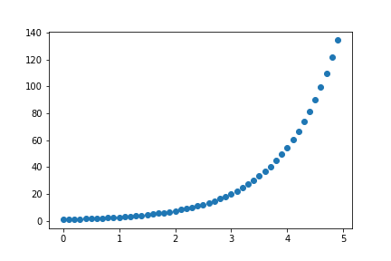
Joyful hallelujah! When making a scatter plot, there’s 3 things you’ll want to concern yourself with:

• point size
• point color
• point edge color

You can control each of these using keyword arguments in plt.scatter(). Let’s alter this plot such that our points are big, red, and don’t have black edges as follows:

In [8]: plt.scatter(x, y, s=50, c="red", edgecolor="None")
        plt.show()

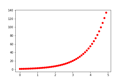
You can also change the point shape using the keyword marker. The available markers are...

• s: Square
• o: Circle
• D: Diamond
• .: Point
• ^, v, >, <: Triangles
• *: Star
• p: Pentagon
• +: Plus signs
• x: X’s
• |: Vertical Lines
• _’: Horizontal Lines

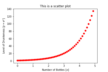
Figures are meaningless without some description of what they’re showing. Every figure should have axis labels.

You can set those labels using the plt.xlabel and plt.ylabel methods. You can also add a title with plt.title

In [9]: plt.title("This is a scatter plot")

        plt.scatter(x, y, s=50, c="red", edgecolor="None")

        plt.xlabel("Number of Bottles [$x$]")

        plt.ylabel("Level of Drunkeness [$y = e^x$]")

        plt.show()

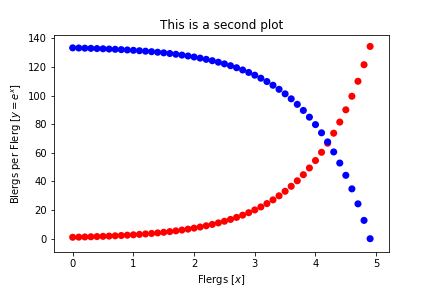
You can also plot two data sets on top of each other. It helps of course to use different colors for each.

In [10]: z = y.max() - y

In [11]: plt.title("This is a second plot")

         plt.scatter(x, y, s=50, c="red", edgecolor="None")

         plt.scatter(x, z, s=50, c="blue", edgecolor="None")

         plt.xlabel("Flergs [$x$]")

         plt.ylabel("Blergs per Flerg [$y = e^x$]")

         plt.show()

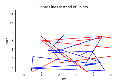
You don’t have to only use numpy arrays to plot your data. If it’s in a simple list, that works too. This time, let’s plot some data as lines instead of points. Let’s also limit the axes so that we’re only looking at a fraction of the data.

In [12]: plt.title("Some Lines Instead of Points")

         the_max = 10
         x1 = [random.randint(0, the_max) for i in range(8)]
         y1 = [random.randint(0, the_max) for i in range(8)]

         x2 = [random.random()*5 for i in range(8)]
         y2 = [random.random()*the_max for i in range(8)]

         plt.plot(x1, y1, color="red")

         plt.plot(x2, y2, color="blue")

         plt.xlabel("Fizz")

         plt.ylabel("Buzz")

         plt.xlim(-0.5, 5)
         plt.ylim(1, 15)

         plt.show()

Typically when we want to simply show the plot without having the repr for the plotting object show up, we use plt.show(). If you want to save the figure to a file, use plt.savefig("relative/or/absolute/path/to/file.png"). You don’t have to save as .png either; a number of image formats including .jpg and even .pdf will work just fine.

Recap

We’re about to step into a different realm of Python, where we consider specifically how to work with data instead of how to serve it for a website. Machine Learning in Python allows us to use the same language we’ve been writing this entire class to make predictions. We can use known data to predict unknown data, or use entirely unknown data to find out interesting insights.

Jupyter Notebook allows us to keep those insights in line with our executable code. We can even style those thoughts with Markdown, giving us a nice interactive environment for experimenting with code.

We can use Python’s powerful Numpy library to do quick math operations and store data in semi-mutable data structures. We can also use Numpy to read data from file into neatly-organized arrays.

Matplotlib affords us the luxury of being able to visualize the data that we have. It’s a massive library so there’s no end to the things it can do, but for our purposes we can use it to plot points and lines to show trends in our data.

Tonight you will get some practice applying these libraries. Tomorrow we’ll meet one more library, Pandas, and learn about how we can clean our data.