Rescaling Data
One issue with classification algorithms is that some of them are biased depending on how close data points are in their parameter space. For example, annual CEO salaries may range between $300 thousand to $30 million, but there isn’t much difference between a CEO making $29 million and one making $30 million. By contrast, length of CEO tenures will often be between 1 - 20 years. I should be able to use both characteristics together to classify CEOs, however if I’m basing my classification on how “close” two data points are in parameter space, the differences of millions in salary will dominate over differences of individual years.
When we use a classification algorithm that relies on distances between points, we need to make sure those distances are on appropriately-similar scales.
Simple Rescaling
The simplest rescaling one can do is to take a range of data and map it onto a zero-to-one scale. Take for example the following data:
In [1]: ages = [44.9, 35.1, 28.2, 19.4, 28.9, 33.5, 22.0, 21.7, 30.9, 27.9]

In [2]: heights = [70.4, 61.7, 75.3, 66.8, 66.9, 61.3, 61.7, 74.4, 76.5, 60.7]

In [3]: import pandas as pd

In [4]: data_df = pd.DataFrame({"ages": ages, "heights": heights})
The range of ages spans across 25.5 years
In [5]: print(data_df.ages.max() - data_df.ages.min())
25.5
while heights (in inches) go across 15.8 inches
In [6]: print(data_df.heights.max() - data_df.heights.min())
15.8
These metrics are clearly not on the same scale. We can put them on the same scale by making their minimum be zero and their maximum be one. The procedure is as follows:
- Subtract from every item in a column the minimum of that column
In [7]: tmp_ages = data_df.ages - data_df.ages.min()
- Divide the resulting values by the maximum of those values.
In [8]: scaled_ages = tmp_ages / tmp_ages.max()

In [9]: print(scaled_ages.min(), scaled_ages.max())
0.0 1.0
Because we always want to avoid changing our source data, let’s make new columns for these rescaled values.
In [10]: tmp_heights = data_df.heights - data_df.heights.min()

In [11]: scaled_heights = tmp_heights / tmp_heights.max()

In [12]: data_df["scaled_ages"] = scaled_ages

In [13]: data_df["scaled_heights"] = scaled_heights
Let’s check that our scaling hasn’t changed the overall distribution of data by visualizing it.
In [14]: import matplotlib.pyplot as plt
In [15]: plt.figure()
Out[15]: <matplotlib.figure.Figure at 0x1076d9da0>
In [16]: plt.subplot(1, 2, 1)
���������������������������������������������������Out[16]: <matplotlib.axes._subplots.AxesSubplot at 0x10b07d0b8>
In [17]: plt.scatter(data_df.ages, data_df.heights)
�������������������������������������������������������������������������������������������������������������������Out[17]: <matplotlib.collections.PathCollection at 0x10acd36a0>
In [18]: plt.xlabel("Ages"); plt.ylabel("Heights")
�����������������������������������������������������������������������������������������������������������������������������������������������������������������������������������Out[18]: <matplotlib.text.Text at 0x10b0e9f60>
In [19]: plt.subplot(1, 2, 2)
����������������������������������������������������������������������������������������������������������������������������������������������������������������������������������������������������������������������������������Out[19]: <matplotlib.axes._subplots.AxesSubplot at 0x107358198>
In [20]: plt.scatter(data_df.scaled_ages, data_df.scaled_heights)
��������������������������������������������������������������������������������������������������������������������������������������������������������������������������������������������������������������������������������������������������������������������������������������������������Out[20]: <matplotlib.collections.PathCollection at 0x107967b38>
In [21]: plt.xlim(0, 1); plt.ylim(0, 1)
������������������������������������������������������������������������������������������������������������������������������������������������������������������������������������������������������������������������������������������������������������������������������������������������������������������������������������������������������������������Out[21]: (0, 1)
In [22]: plt.xlabel("Scaled Ages"); plt.ylabel("Scaled Heights")
����������������������������������������������������������������������������������������������������������������������������������������������������������������������������������������������������������������������������������������������������������������������������������������������������������������������������������������������������������������������������������Out[22]: <matplotlib.text.Text at 0x10b717940>
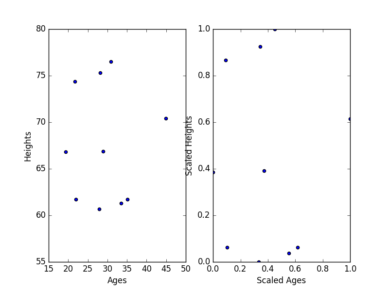
And now you’ve got the same distribution of data, but rescaled in such a way that distances between points won’t be biased by differences in scale.
This technique is called Min-Max Scaling.
Python’s scikit-learn library has a tool just for this called the MinMaxScaler.
You can use that to rescale your values as well, if you’d like.
In [23]: from sklearn.preprocessing import MinMaxScaler

In [24]: scaler = MinMaxScaler()

In [25]: scaled_ages = scaler.fit_transform(data_df.ages)

In [26]: print(scaled_ages)
Out[26]:
array([ 1.        ,  0.61568627,  0.34509804,  0.        ,  0.37254902,
    0.55294118,  0.10196078,  0.09019608,  0.45098039,  0.33333333])
Orders of Magnitude
Sometimes data spans across many powers of 10. A great example is annual income. Looking at people in the United States, some folks (e.g. graduate students) make around $20,000 per year (\(2\times10^4\)) while some CEOs make upwards of $100 million annually (\(1\times10^8\)). That’s 4 orders of magnitude (powers of 10) in difference! Any other comparison that doesn’t span that same range of numbers will get washed out easily. Let’s see this with some data.
In [27]: salaries = [1000.0, 3593.8, 12915.5, 46415.9, 166810.1, 599484.3, 2154434.7, 7742636.8, 27825594.0, 100000000.0]

In [28]: scaler = MinMaxScaler()

In [29]: scaled_salaries = scaler.fit_transform(salaries)

In [30]: print(scaled_salaries)
[  0.00000000e+00   2.59383960e-05   1.19156158e-04   4.54163425e-04
   1.65811712e-03   5.98490235e-03   2.15345622e-02   7.74171424e-02
   2.78248723e-01   1.00000000e+00]
If we use the same MinMaxScaler we used above, the scaling doesn’t really do much for making this range manageable.
When we have data that goes across such a large dynamic range, we need to get a little fancy to make these values workable with our distance calculations.
Logarithms
In math, a logarithm is the number (\(x\)) to which some base number (\(b\)) must be raised to produce the number we see (\(y\)).
So if our base is 10, then to get to 100 million, we have to raise 10 to the power 8. Thus, \(\log_{10}(100,000,000) = 8\). That function, \(\log_{10}\) takes in a number and returns the power of 10 it corresponds to.
In [31]: import numpy as np

In [32]: np.log10(10000)
Out[32]: 4.0

In [33]: 10**4.0
Out[33]: 10000

In [34]: np.log10(30)
Out[34]: 1.4771212547196624

In [35]: 10**_
Out[35]: 29.999999999999996 # issues with floats but you get the point

In [36]: salaries = np.array(salaries)

In [37]: np.log10(salaries)
Out[37]:
array([ 3.        ,  3.55555556,  4.11111111,  4.66666667,  5.22222222,
        5.77777778,  6.33333333,  6.88888889,  7.44444444,  8.        ])
In that last line we’ve rescaled the salaries logarithmically. Now these values are more linear, and we can apply our standard MinMax scaling for use in our distance calculations.
No matter which method you use, make it appropriate for your data. There are of course many more steps you can take, but these are good enough for now. Always inspect first, then decide on a preprocessing step.