Statistics 2: Probability, Distributions, & Tests¶

Package/module refs:

pandas for storing your data
numpy also for storing data (as arrays), and other awesome things
math.factorial for factorials
scipy.stats for t-tests and distribution functions
matplotlib.pyplot for visualizing your data
my tutorial on plotting data. It’s focused on Astronomy but is universally (HA!) applicable

Handling Null Data¶

No dataset is perfect. Most data that you work with, especially human-compiled data, will be somewhat incomplete. Missing values. When incomplete data is loaded with pandas.read_csv, numpy.loadtxt, or numpy.genfromtxt, those missing pieces will be filled by a default NaN (not a number) value.

In [1]:

import pandas as pd
import numpy as np

incomplete_data = pd.read_csv("../downloads/nmhw_sample_data.csv")
incomplete_data

Out[1]:

	Name	Age	Hometown	Country	Desired Income	Favorite Food	Number of Cats
0	James	22	New York	NaN	75000.0	NaN	0.0
1	Bob	25	Seattle	USA	0.0	pad thai	2.0
2	Annette	28	San Francisco	USA	NaN	spaghetti	1.0
3	Florence	23	Beijing	China	60000.0	xiaolong bao	4.0
4	Martha	30	Kansas City	NaN	NaN	corn	3.0
5	Desean	27	Newark	USA	85000.0	NaN	NaN
6	Jamal	28	New York	NaN	65000.0	pizza	3.0
7	Kaede	31	Kyoto	Japan	65000.0	sushi	4.0
8	Milton	23	Austin	NaN	78000.0	bbq	NaN
9	Ivana	29	Moscow	Russia	NaN	borscht	1.0
10	Jorge	35	Rio de Janeiro	Brasil	90000.0	farofa	2.0

Always keep in mind that a “NaN” value *only* signifies a non-entry. Often, it’s tempting to just replace NaN values with zeros, or False, but to universally assume that you can or even should do that doesn’t do justice to what a NaN is. To be sure, NaN values *are numerical* but neither represent any actual number nor evaluate as False, None, or infinity.

In [2]:

this_val = incomplete_data.Country.iloc[0]
print(this_val)
print(type(this_val))
print((this_val == 0) | (this_val < 0) | (this_val > 0) | (this_val == np.inf))
print((this_val == False) | (this_val == None))
if this_val:
    print("This still prints something because it still represents a thing.")

nan
<class 'float'>
False
False
This still prints something because it still represents a thing.

There are many ways to handle NaN values and many entries (or lackthereof) that should be recognized as such. Pandas allows you to recognize a variety of values as null upon entry with the na_values parameter of pandas.read_csv

In [3]:

incomplete_data = pd.read_csv("../downloads/nmhw_sample_data.csv", na_values=["null", "NULL", -9999, np.inf])

Once assigned to a variable, NaN values can be dealt with on a column-by-column basis or throughout the entire DataFrame with the fillna method. A NaN might be set to some default value, as you may be able to assume a meaningful value for a non-entry. You may also decide that a different column’s NaN may need to be evaluated in order to get it out of the way in filtering or some other data process later on.

In [4]:

incomplete_data.Country.fillna("USA")

Out[4]:

      USA
      USA
      USA
    China
      USA
      USA
      USA
    Japan
      USA
   Russia
  Brasil
Name: Country, dtype: object

In [5]:

print(incomplete_data["Number of Cats"].fillna(-99))

0      0.0
1      2.0
2      1.0
3      4.0
4      3.0
5    -99.0
6      3.0
7      4.0
8    -99.0
9      1.0
10     2.0
Name: Number of Cats, dtype: float64

If your data is ordered, you can use the “method” parameter to fill NaNs with the last seen value with method=ffill or with the next valid data point method=bfill

In [6]:

incomplete_data.fillna(method="ffill")

Out[6]:

	Name	Age	Hometown	Country	Desired Income	Favorite Food	Number of Cats
0	James	22	New York	NaN	75000.0	NaN	0.0
1	Bob	25	Seattle	USA	0.0	pad thai	2.0
2	Annette	28	San Francisco	USA	0.0	spaghetti	1.0
3	Florence	23	Beijing	China	60000.0	xiaolong bao	4.0
4	Martha	30	Kansas City	China	60000.0	corn	3.0
5	Desean	27	Newark	USA	85000.0	corn	3.0
6	Jamal	28	New York	USA	65000.0	pizza	3.0
7	Kaede	31	Kyoto	Japan	65000.0	sushi	4.0
8	Milton	23	Austin	Japan	78000.0	bbq	4.0
9	Ivana	29	Moscow	Russia	78000.0	borscht	1.0
10	Jorge	35	Rio de Janeiro	Brasil	90000.0	farofa	2.0

In [7]:

incomplete_data.fillna(method="bfill")

Out[7]:

	Name	Age	Hometown	Country	Desired Income	Favorite Food	Number of Cats
0	James	22	New York	USA	75000.0	pad thai	0.0
1	Bob	25	Seattle	USA	0.0	pad thai	2.0
2	Annette	28	San Francisco	USA	60000.0	spaghetti	1.0
3	Florence	23	Beijing	China	60000.0	xiaolong bao	4.0
4	Martha	30	Kansas City	USA	85000.0	corn	3.0
5	Desean	27	Newark	USA	85000.0	pizza	3.0
6	Jamal	28	New York	Japan	65000.0	pizza	3.0
7	Kaede	31	Kyoto	Japan	65000.0	sushi	4.0
8	Milton	23	Austin	Russia	78000.0	bbq	1.0
9	Ivana	29	Moscow	Russia	90000.0	borscht	1.0
10	Jorge	35	Rio de Janeiro	Brasil	90000.0	farofa	2.0

You can choose to fill with the mean or median, however take note that strings can’t be averaged or median-ed. So be aware of what columns you’re fiddling with.

In [8]:

incomplete_data["Age"].fillna(incomplete_data.mean()["Age"])

Out[8]:

   22
   25
   28
   23
   30
   27
   28
   31
   23
   29
  35
Name: Age, dtype: int64

In [9]:

incomplete_data["Desired Income"].fillna(incomplete_data.median()["Desired Income"])

Out[9]:

   75000.0
       0.0
   70000.0
   60000.0
   70000.0
   85000.0
   65000.0
   65000.0
   78000.0
   70000.0
  90000.0
Name: Desired Income, dtype: float64

Other times it would make more sense to just leave NaNs as they are. Aggregate operations like means and sums will just ignore them. Though be aware that they will screw up iterative processes with strings.

In [10]:

print(incomplete_data["Desired Income"].mean())
incomplete_data["Favorite Food"].map(lambda x: x.split(" "))

64750.0

---------------------------------------------------------------------------
AttributeError                            Traceback (most recent call last)
<ipython-input-10-89f3d5c32e54> in <module>()
      1 print(incomplete_data["Desired Income"].mean())
----> 2 incomplete_data["Favorite Food"].map(lambda x: x.split(" "))

/Users/Nick/anaconda/envs/python-dev-accelerator/lib/python3.5/site-packages/pandas/core/series.py in map(self, arg, na_action)
   2119                                      index=self.index).__finalize__(self)
   2120         else:
-> 2121             mapped = map_f(values, arg)
   2122             return self._constructor(mapped,
   2123                                      index=self.index).__finalize__(self)

pandas/src/inference.pyx in pandas.lib.map_infer (pandas/lib.c:63043)()

<ipython-input-10-89f3d5c32e54> in <lambda>(x)
      1 print(incomplete_data["Desired Income"].mean())
----> 2 incomplete_data["Favorite Food"].map(lambda x: x.split(" "))

AttributeError: 'float' object has no attribute 'split'

It’s worth noting that while NaN values essentially mean the same no matter what, not all NaNs are created equal. A pandas nan is not the same as a numpy nan (although oddly-enough will be recognized as a nan-like value), and vice versa.

In [11]:

print(this_val == np.nan)
print(np.isnan(this_val))
print(pd.isnull(np.nan))
print(type(np.nan))

False
True
True
<class 'float'>

At the end of the day, no matter what you decide to do with NaNs make sure that you know your data and have an idea of what you want to do with it. All choices will follow from the nature of your data set and what your analysis entails.

Basic Rules of Probability¶

The chance that some event happens given all events that could happen in that category.
Probabilities denote the chance that something happens, not the guarantee
$0 \le p(x) \le 1$ or $0\% \le p(x) \le 100\%$
For any set of associated but separate events, $\displaystyle\sum_i p(x_i) = 1$
For related events A and B, the probablity that they happen together is

$p(A \cap B) = p(A) \cdot p(B)$

The probability that either one of them happens is

$p(A \cup B) = p(A) + p(B) - p(A \cap B)$

Examples:¶

p(coin toss = Head)
p(rolling D20 and getting ≤ 11)
p(5 coin tosses = Head)
For bag of 4 white balls and 6 black balls, p(drawing 2 white then 2 black)

Probability Distributions¶

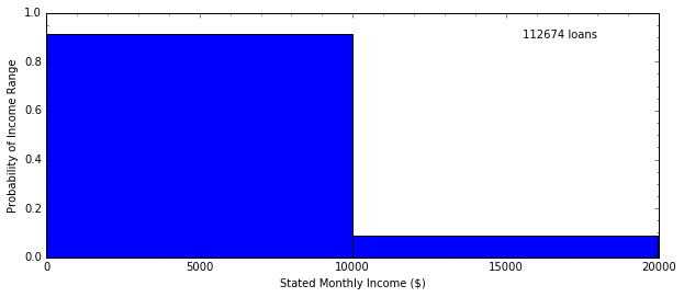
In [12]:

import matplotlib.pyplot as plt
%matplotlib inline

data = pd.read_csv("../downloads/prosperLoanData_truncated.csv", sep=",")
data = data[data.StatedMonthlyIncome < 2E4]
H, edges = np.histogram(data.StatedMonthlyIncome, bins=2)

plt.figure(figsize=(10, 4))
ax = plt.subplot(111)
ax.bar(edges[:-1], H / float(sum(H)), width=edges[1] - edges[0])
ax.text(0.9, 0.9, "%g loans" % len(data),
        horizontalalignment="right", transform=ax.transAxes)
ax.set_xlabel("Stated Monthly Income ($)")
ax.set_ylabel("Probability of Income Range")
ax.minorticks_on()
plt.show()

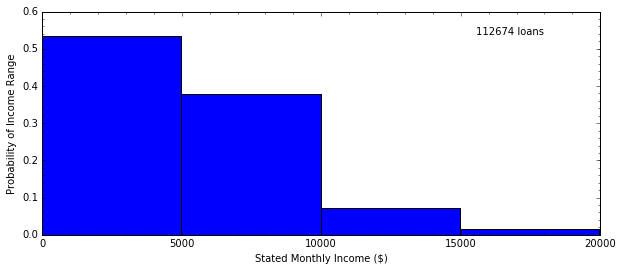
In [13]:

H, edges = np.histogram(data.StatedMonthlyIncome, bins=4)

plt.figure(figsize=(10, 4))
ax = plt.subplot(111)
ax.bar(edges[:-1], H / float(sum(H)), width=edges[1] - edges[0])
ax.text(0.9, 0.9, "%g loans" % len(data),
        horizontalalignment="right", transform=ax.transAxes)
ax.set_xlabel("Stated Monthly Income ($)")
ax.set_ylabel("Probability of Income Range")
ax.minorticks_on()
plt.show()

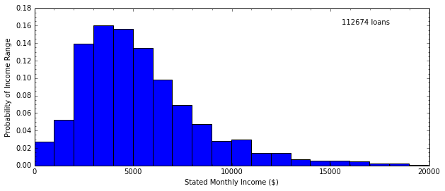
In [14]:

H, edges = np.histogram(data.StatedMonthlyIncome, bins=20)

plt.figure(figsize=(10, 4))
ax = plt.subplot(111)
ax.bar(edges[:-1], H / float(sum(H)), width=edges[1] - edges[0])
ax.text(0.9, 0.9, "%g loans" % len(data),
        horizontalalignment="right", transform=ax.transAxes)
ax.set_xlabel("Stated Monthly Income ($)")
ax.set_ylabel("Probability of Income Range")
ax.minorticks_on()
plt.show()

In [15]:

H, edges = np.histogram(data.StatedMonthlyIncome, bins=50)

plt.figure(figsize=(10, 4))
ax = plt.subplot(111)
ax.bar(edges[:-1], H / float(sum(H)), width=edges[1] - edges[0])
ax.text(0.9, 0.9, "%g loans" % len(data),
        horizontalalignment="right", transform=ax.transAxes)
ax.set_xlabel("Stated Monthly Income($)")
ax.set_ylabel("Probability of Income Range")
ax.minorticks_on()
plt.show()

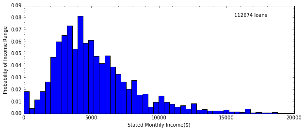
Note that here I use ax to access the plot space of the figure, so that I can place text wherever I want it. If I don’t use the transform parameter, then if I want to place text on a figure I have to specify the exact coordinates in the data space for where I want it to be. With transforming to the coordinate space of the figure, I can use the fact that coordinate space goes from 0 to 1 horizontally and vertically to place text easily.

One issue is that if you use ax, you set axis labels using ax.set_xlabel and ax.set_ylabel instead of the normal methods with plt.xlabel and plt.ylabel. Similar for setting axis limits.

Also note that with numpy arrays (and pandas DataFrames), you can perform arithmetic on the entire object at once. Also note that with numpy arrays specifically, you cannot alter the size of the array once it’s been created. Fixed-size arrays make it faster, but the immutability of size can be a little difficult. At least you can alter the values inside the array easily through indexing.

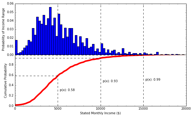
Cumulative Probability Distribution¶

The probability of getting a value less than x

In [16]:

H, edges = np.histogram(data.StatedMonthlyIncome, bins=np.linspace(0, 2E4, 81))
incomes = [5000, 10000, 15000]

fig = plt.figure(figsize=(10, 6))
fig.subplots_adjust(hspace=0) # smooshes vertical subplots together
ax = plt.subplot(211) # 2 rows, 1 column, put this figure in the first cell
ax.bar(edges[:-1], H / float(sum(H)), width=edges[1] - edges[0])
for ii in incomes:
    ax.plot([ii, ii], [0, 0.06], linestyle="--", color='k')
ax.set_ylabel("Probability of Income Range")
ax.set_xticklabels([]) # kills the numbers on the x-axis for this plot
ax.minorticks_on()

ax = plt.subplot(212) # 2 rows, 1 column, put this figure in the first cell
probabilities = H.cumsum() / float(sum(H))
ax.plot(edges[:-1], probabilities, linewidth=5, color="r")
for ii in incomes:
    prob = probabilities[edges[:-1] == ii]
    ax.plot([ii, ii], [0, prob], linestyle="--", color='k')
    ax.plot([0, ii], [prob, prob], linestyle="--", color='k')
    ax.text(ii + 2.5E2, prob * 0.5, "p(x): %.2f" % prob)
ax.set_xlabel("Stated Monthly Income ($)")
ax.set_ylabel("Cumulative Probability")
ax.set_ylim(0, 0.99)
ax.minorticks_on()
plt.savefig("../downloads/cumulative_distribution.png")
plt.show()

Numpy arrays have several methods, one of which is cumsum(). This method performs a cumulative sum on your array from left to right.

arr = np.array([1, 1, 1, 1, 1, 1, 1, 1])
arr.cumsum()
>>> array([1, 2, 3, 4, 5, 6, 7, 8])

“If I choose a person from this data set at random, there’s a 58% chance that their monthly salary is less than $5,000”
”..., there’s a 35% chance their monthly salary is between $5,000 and $10,000”
”..., there’s a 1% chance their monthly salary is greater than $15,000”

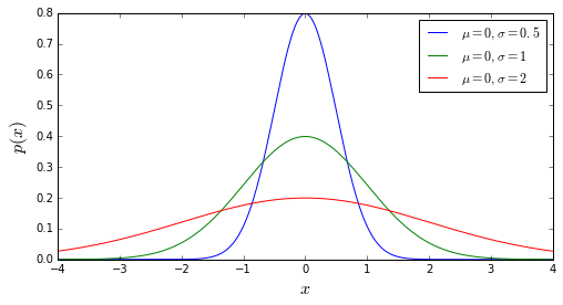
The Gaussian/Normal Distribution¶

Theoretical curve describing the probability of getting some value x, given the mean and standard deviation of the data
$p(x|\sigma, \mu) = \displaystyle\frac{1}{\sqrt{2\pi\sigma^2}}\exp{\left[\frac{-(x - \mu)^2}{2\sigma^2}\right]}$
The most commonly-used distribution
Ref: Central Limit Theorem
The Gist: The mean of samples drawn from an almost arbitrary distribution will approx. follow a Gaussian
Applied to everything, even when not appropriate

In [17]:

del data

def gaussian(x, mu, std):
    return (1. / np.sqrt(2 * np.pi * std**2) * np.exp(-0.5 * ((x - mu) / std)**2))
x = np.linspace(-4, 4, 1000)
fig = plt.figure(figsize=(8, 4))
plt.plot(x, gaussian(x, 0, 0.5), label="$\mu = 0, \sigma = 0.5$")
plt.plot(x, gaussian(x, 0, 1), label="$\mu = 0, \sigma = 1$")
plt.plot(x, gaussian(x, 0, 2), label="$\mu = 0, \sigma = 2$")
plt.xlabel("$x$", fontsize=16)
plt.ylabel("$p(x)$", fontsize=16)
plt.legend()
plt.savefig("../downloads/gaussian_distribution.png")
plt.show()

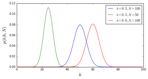
The Binomial Distribution¶

Describes the distribution of a variable that can only take two values (0/1, False/True, Heads/Tails)
For N trials...
I know the probability b of getting one outcome per trial...
I can describe the probability of getting k successes of that outcome:

\[p(k|b,N) = \displaystyle\frac{N!}{k!(N-k)!}b^k(1 - b)^{N-k}\]

The mean $\bar{k} = b\,N$
The standard deviation $\sigma_k = \sqrt{N \,b \,(1 - b)}$
NOTE: does not describe probability of getting consecutive successes or any particular combination of successes & failures

In [18]:

from math import factorial


def binomial(k, N, b):
    return float(factorial(N)) / (factorial(k) * factorial(N - k)) * b ** k * (1 - b)**(N - k)

x = range(1, 100)
y0 = [binomial(val, 100, 0.5) for val in x]
y1 = [binomial(val, 50, 0.5) for val in range(0, 50)]
y2 = [binomial(val, 100, 0.6) for val in x]
fig = plt.figure(figsize=(8, 4))
plt.plot(x, y0, label="$b = 0.5, N = 100$")
plt.plot(range(0, 50), y1, label="$b = 0.5, N = 50$")
plt.plot(x, y2, label="$b = 0.6, N = 100$")
plt.xlabel("$k$", fontsize=16)
plt.ylabel("$p(k | b, N)$", fontsize=16)
plt.legend()
plt.savefig("../downloads/binomial_distribution.png")
plt.show()

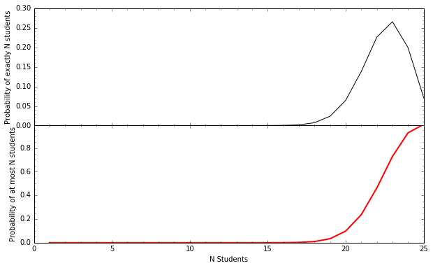
Example: the probability of $\ge k$ Code Fellows students getting a job after 6 months¶

In [19]:

from scipy.stats import binom

n_students = np.arange(1, 26)
total_students = 25
prob_of_success = 0.9
individual_probability = [binom.pmf(x, total_students, prob_of_success) for x in n_students]
cumulative_probability = [binom.cdf(x, total_students, prob_of_success) for x in n_students]

fig = plt.figure(figsize=(10, 6))
fig.subplots_adjust(hspace=0)

ax = plt.subplot(211)
ax.plot(n_students, individual_probability, color="k")
ax.set_xticklabels([])
ax.set_ylabel("Probability of exactly N students")
ax.minorticks_on()

ax = plt.subplot(212)
ax.plot(n_students, cumulative_probability, color="r", linewidth=2)
ax.set_xlabel("N Students")
ax.set_ylabel("Probability of at most N students")
ax.set_ylim(0, 0.99)
ax.minorticks_on()

plt.show()

Hypothesis Testing and Measurement Significance¶

Chance occurrence vs meaningful occurrence
Sticking with the Gaussian distribution of random samples
Either reject the Null Hypothesis $H_0$ or fail to reject it.
Can never PROVE absolutely True or absolutely False
Hypothesis conclusions entirely dependent on the sample. Cannot be assumed to be universal.
Significance levels ($\alpha$) help decide whether to reject $H_0$
- Typical $\alpha$-levels: 0.05, 0.025, 0.01
Statistical tests produce two things:
- a numerical statistic showing the distance between the means of two distributions (more later)
- a “p-value” showing the probability of getting this result given the null hypothesis
If your p-value is less than some alpha-level, then it’s statistically significant to that level
- ex: p = 0.035; my test rejects the null hypothesis at $\alpha = 0.05$ significance level, but not at the $\alpha = 0.025$ level.
- ex: p = 0.13; my tests fails to reject the null hypothesis

Students’ t-Test¶

“Students” was the pseudonym of the originator
Computes a statistic (the “t” statistic) based on the means and variances of samples

\[t = \displaystyle\frac{\bar{x_1} - \bar{x_2}}{\sqrt{\frac{s_1^2}{n_1} + \frac{s_2^2}{n_2}}}\]
Defs:
- $s_i$: standard deviation of sample $i$
- $n_i$: number of items in sample $i$
Use Cases
- test whether a subsample is significantly different from the population
- test if two subsamples from the same population are significantly different
- test if two independent samples are significantly different
Note: Data should be somewhat “normally” distributed (so visualize). Non-normal data needs a different test (next time

t-Test example: Seattle Weather in 2010¶

Hypothesis: The temperature during the Spring was significantly different than the temperature during the Fall
Null hypothesis: The temperature during the Spring wasn’t significantly different
Define terms:
- Spring: March through May
- Fall: September through November

In [20]:

import os

data_dir = "../downloads/seattle_weather/"
weather_files = [
    data_dir + f for f in os.listdir(data_dir) if f.startswith("MonthlyHistory")]
seattle_weather = pd.read_csv(weather_files[0])

for f in weather_files[1:]:
    indata = pd.read_csv(f)
    if "PDT" in indata.columns:
        indata.rename(columns={'PDT': 'PST'}, inplace=True)

    seattle_weather = pd.concat((seattle_weather, indata), ignore_index=True)

pandas.concat takes two DataFrames and merges them into one DataFrame. If you don’t set ignore_index=True then it will preserve the index values that each individual DataFrame had before merging, which can become problematic when slicing the new merged frame

Note that when concatenating DataFrames, any columns that exist in one and not in the other will get filled with null values. Above, I just change the name of the “PDT” column because not every data file has that column despite them all showing roughly the same data.

In [21]:

seattle_weather["year"] = seattle_weather.PST.map(lambda x: float(x.split("-")[0]))
seattle_weather["month"] = seattle_weather.PST.map(lambda x: float(x.split("-")[1]))
seattle_weather["day"] = seattle_weather.PST.map(lambda x: float(x.split("-")[2]))

You can create new columns in a DataFrame much like how you can create new keys in a dictionary, by specifying the column name that you want. You can also get data from columns in two ways: calling that column up with the square bracket notation DataFrame["column_name"] or with dot notation DataFrame.column_name. The main difference is that dot notation cannot handle column names with spaces.

In [22]:

spring_2010 = (seattle_weather.year == 2010) & (seattle_weather.month > 2) & (seattle_weather.month < 6)
fall_2010 = (seattle_weather.year == 2010) & (seattle_weather.month > 8) & (seattle_weather.month < 12)

You can select indices of data matching specific criteria. The above lines produce two pandas Series objects (effectively a one-column DataFrame) holding boolean values of True when a row matches your criteria, and False when it doesn’t. You can do the same with numpy arrays (where the same selection will produce numpy arrays filled with booleans)

In [23]:

plt.figure(figsize=(10, 4))
opacity = 0.5
mean_temp = "Mean TemperatureF"
plt.hist(seattle_weather[spring_2010][mean_temp], bins=np.arange(20, 76, 4), alpha=opacity, label="Spring 2010")
plt.hist(seattle_weather[fall_2010][mean_temp], bins=np.arange(20, 76, 4), alpha=opacity, label="Fall 2010")
plt.legend()
plt.xlabel("Mean Temperature (F)")
plt.ylabel("N days")
plt.show()

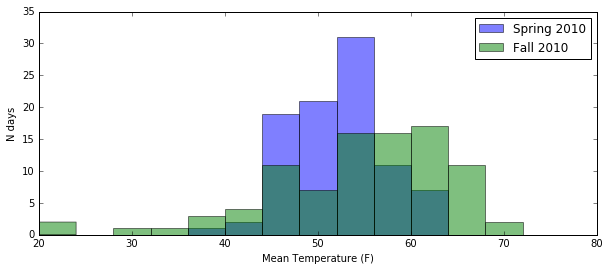
The alpha parameter controls the opacity of whatever you’re plotting, whether they are bars, points, lines, circles, whatever. Opacity goes from 0 to 1. Works best when you you have heavily overlapping data. In the event of overlapping data, plot the larger data set first (in the background) so that it doesn’t drown out the smaller set.

In [24]:

from scipy.stats import ttest_ind

t_stat, p_value = ttest_ind(seattle_weather[spring_2010][mean_temp],
                            seattle_weather[fall_2010][mean_temp])
print("Results:\n\tt-statistic: %.5f\n\tp-value: %.5f" % (t_stat, p_value))

Results:
        t-statistic: -2.09063
        p-value: 0.03796

I can reject the null hypothesis at the p < 0.05 significance level. At that level, the mean temperature in Spring and Fall 2010 was significantly different.

t-tests in SciPy.stats¶

`ttest_ind <http://docs.scipy.org/doc/scipy-0.16.0/reference/generated/scipy.stats.ttest_ind.html#scipy.stats.ttest_ind>`__: performs a t-test on two sample distributions and returns the t-statistic (useful later) and the p-value; useful for two independent samples from the same population (or very similar but different populations)
`ttest_1samp <http://docs.scipy.org/doc/scipy-0.16.0/reference/generated/scipy.stats.ttest_1samp.html#scipy.stats.ttest_1samp>`__: useful for one sample distribution in comparison to the mean of a population
`ttest_rel <http://docs.scipy.org/doc/scipy-0.16.0/reference/generated/scipy.stats.ttest_rel.html#scipy.stats.ttest_rel>`__: useful for two related samples